Dorsey, Bailee ¹ ; de Meeûs, Thierry ² ; Allerdice, Michelle E. J. ³ ; Paddock, Christopher D. ⁴ ; Nicholson, William L. ⁵ ; Ayres, Bryan N. ⁶ ; Wisely, Samantha M. ⁷ ; Noden, Bruce H. ⁸ and Beati, Lorenza ⁹

¹The U.S. National Tick Collection, ICPS, Georgia Southern University, Statesboro, Georgia, U.S.A.
²Intertryp, Univ Montpellier, Cirad, IRD, Montpellier, France.
³Rickettsial Zoonoses Branch, Centers for Disease Control and Prevention, Atlanta, Georgia, U.S.A.
⁴Rickettsial Zoonoses Branch, Centers for Disease Control and Prevention, Atlanta, Georgia, U.S.A.
⁵Rickettsial Zoonoses Branch, Centers for Disease Control and Prevention, Atlanta, Georgia, U.S.A.
⁶Rickettsial Zoonoses Branch, Centers for Disease Control and Prevention, Atlanta, Georgia, U.S.A.
⁷Department of Wildlife Ecology and Conservation, University of Florida, Gainesville, Florida, U.S.A.
⁸Department of Entomology and Plant Pathology, Oklahoma State University, Oklahoma, U.S.A.
⁹✉ The U.S. National Tick Collection, ICPS, Georgia Southern University, Statesboro, Georgia, U.S.A.

2025 - Volume: 65 Issue: 2 pages: 519-533

Original research

Keywords

Abstract

Introduction

The Gulf Coast tick, Amblyomma maculatum Koch, 1844 (Acari: Ixodidae) belongs to the A. maculatum species group, which also includes Amblyomma tigrinum Koch, 1844 and Amblyomma triste Koch, 1844 (Kohls 1956; Estrada-Peña et al. 2005). In the United States, the geographic range of A. maculatum has expanded northward during the past two decades. Through most of the 20^th century, the recognized U.S. distribution of A. maculatum included a relatively narrow, but contiguous region lying approximately 200 km inward from the southeast coast, and extending from Texas to South Carolina (Cooley and Kohls 1944; Kohls 1956; Paddock and Goddard 2015). Established populations now exist in many northeastern states, including Connecticut, Delaware, New Jersey and New York, as well as several inland central states, including Arkansas, Illinois, Kansas, and Oklahoma (Trout et al. 2010; Florin et al. 2014; Paddock and Goddard 2015; Sonenshine 2018; Phillips et al. 2020; Molaei et al. 2021; Bajwa et al. 2022; Ramírez-Garofalo et al. 2022). The range expansion has been ascribed in part to climate change (Sonenshine 2018; Alkishe and Peterson 2022), and phoretic expansion on migratory birds to reestablished grassland habitats in the eastern United States (Paddock and Goddard 2015; Ramírez-Garofalo et al. 2022). Indeed, A. maculatum s.l. is known to parasitize avian hosts as immatures and to be carried by migratory birds in the U.S. and Canada (Cooley and Kohls 1944; Keirans and Durden 1998; Teel et al. 1998; Kinsey, Durden and Oliver 2000; Estrada-Peña et al. 2005; Mukherjee et al. 2014; Bajwa et al. 2022; Flenniken et al. 2022; Scott, McKeown and Scott 2023). Nadolny and Gaff (2018) stated that birds and large to medium sized animals, including dogs traveling with their owners, are contributing to the range expansion of A. maculatum. Cattle movements across the U.S. have also been mentioned as a possible source of newly established populations (Semtner and Hair 1973; Teel et al. 2010; Trout et al. 2010).

Ticks identified as A. triste, one of the other recognized taxa in the A. maculatum species group, were described recently from archival specimens obtained from birds and mammals in southern Arizona, western Texas, and northern Mexico (Guzmán-Cornejo et al. 2006; Mertins et al. 2010). These ticks were identified based on their adult tibiotarsal armature, ornamentation, and punctation patterns reminiscent of A. triste. Nevertheless, a subsequent morphological examination of field-collected, host-seeking specimens obtained from multiple sites in southern Arizona (Allerdice et al. 2017) and northern Mexico (Delgado de la Mora et al. 2019), as well as A. triste from Argentina, A. maculatum s.l. from Peru, and A. maculatum s.s. from the eastern U.S. identified four distinct morphotypes: morphotype I corresponded to A. triste sensu stricto (s.s.) from Argentina and Uruguay, morphotype II to A. maculatum s.s. from the eastern U.S., morphotype III to the ticks from Arizona and northern Mexico, and morphotype IV to the Peruvian specimens (Lado et al. 2018). Morphotypes III and IV had intermediary morphological features between A. triste s.s. and A. maculatum s.s. and differed from each other. This biogeographic distribution does not preclude the possibility that real A. triste specimens could sporadically be imported into the U.S. on migratory birds, particularly because A. triste s.s. has now been detected as far north as Colombia (Ossa-López et al. 2022). Nevertheless, all observations indicate that contemporary field-collected specimens obtained in Arizona and northern Mexico differ markedly from A. triste s.s. (Lado et al. 2018). More recently, specimens of morphotype III have been collected from multiple sites in southern New Mexico (Hecht et al. 2020) and west Texas (Paddock et al. 2020).

Molecular phylogenetic analyses (Lado et al. 2018) based on both mitochondrial and nuclear (ITS2) datasets revealed that the A. maculatum group consists of four well-resolved lineages: A. tigrinum, A. triste s.s. (morphotype I), the Peruvian clade (morphotype IV), and a last clade clustering A. maculatum s.s from the eastern U.S (morphotype II), the southwestern U.S., and Mexico (morphotype III). Because morphotypes II and III did not segregate into two mutually exclusive lineages, the study could not confirm that these were in fact two different species. This study also showed that the A. maculatum group radiated and speciated very recently (Lado et al. 2018) compared to other Amblyomma groups with similar geographical distributions (Beati et al. 2013).

Crossbreeding experiments were subsequently performed to further investigate if morphotypes II and III were two distinct species (Allerdice et al. 2020). This study showed that while the two morphotypes could easily crossbreed and generate live offspring, F1 hybrid females produced non-viable eggs. This result supported the existence of two different species. Rickettsia parkeri Lackman, 1965, a pathogenic spotted fever group Rickettsia species, has been detected extensively in morphotypes I, II, and III of the A. maculatum tick group (Nava et al. 2008; Paddock et al. 2010; Delgado-de la Mora et al. 2017; Allerdice et al. 2017; Hecht et al. 2020; Paddock et al. 2020). A recent molecular analysis of R. parkeri isolates from the Western Hemisphere revealed a genotype unique to morphotype III that was not found in morphotype II, providing additional support for a separate evolutionary history of the two morphotypes (Allerdice et al. 2021).

Microsatellite markers are known to mutate rapidly compared to the coding gene sequences used commonly for taxonomic reassessments. Because of their high mutation rates, these markers can provide sensitive tools not only for population genetic structure studies, but also for species delimitation, particularly for recent or ongoing speciation events (De Meeûs et al. 2010; Manangwa et al. 2019), which appears to be the case for the A. maculatum species group (Lado et al. 2018). Microsatellite markers have been developed for several tick species and genera and have successfully supplied information on population structure, dispersal patterns, mating behavior, tick-host associations, and taxonomy (De Meeûs et al. 2002; McCoy, Tirard and Michalakis 2003; Hasle, Røed and Leinaas 2008; Labruna et al. 2009; Kempf et al. 2011; Ogrzewalska et al. 2014; Velez et al. 2023). In this study, eight previously selected microsatellite loci (Allerdice 2021) were tested on natural populations of the A. maculatum group collected in 2016 from the eastern and western U.S. populations of morphotypes II and III. The main goal was to verify if the analysis of microsatellite loci would provide support for the occurrence of two species. In addition, these markers were used for a preliminary study of the genetic structure of the group, an evaluation of the divergence time of the two morphotypes, and to estimate their respective per generation dispersal distances.

Material and methods

Samples

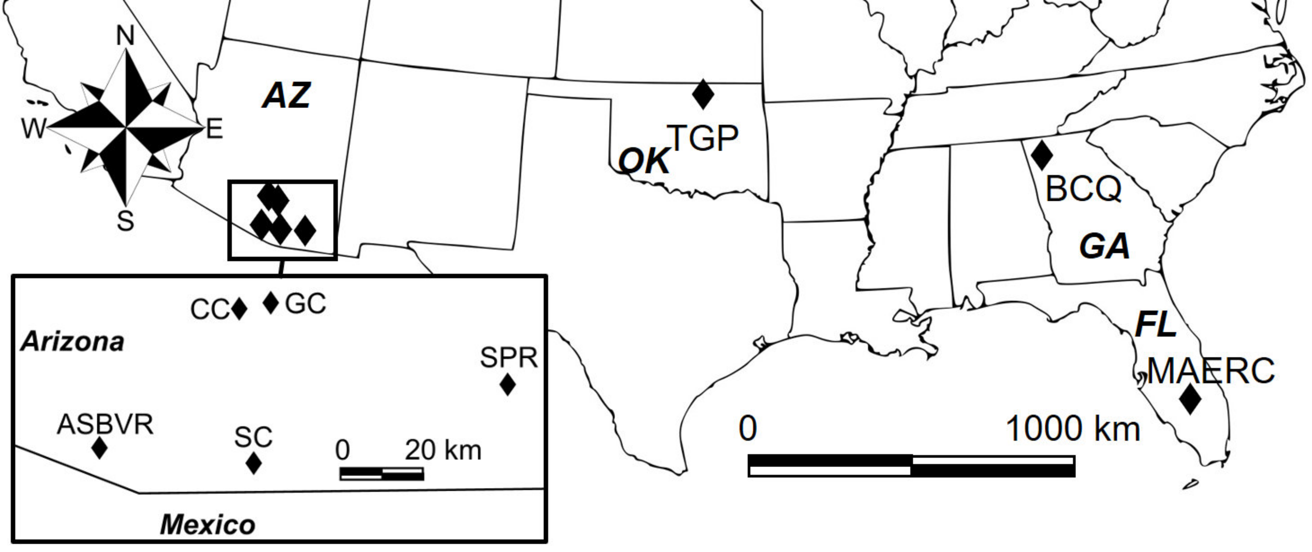
Male and female A. maculatum s.s. (morphotype II) and morphotype III ticks were sampled from various sites across the U.S. from May to July 2016 by dragging the vegetation or inspecting cattle. Collection sites are shown in Figure 1, with additional information in Table 1.

Selection and characterization of microsatellite markers

The methods used to select microsatellite loci are described elsewhere in detail (Allerdice 2021). Because of the important stuttering issues encountered in another tick species when trying to score dinucleotide loci (De Meeûs et al. 2021), only tri- and tetranucleotide tandem repeat loci, with no more than 1-2 copies/genome were used. Eight loci were selected based on high polymorphism and the apparent absence of null alleles (Allerdice 2021). Of these, four were trinucleotide repeats (L12, L19, L20, and L53) and four were tetranucleotide repeats (L74, L91, L103, and L112) (Table 2).

Genotyping

DNA was extracted from samples following a previously described method that allows for the simultaneous preservation of tick exoskeletons (Beati and Keirans 2001). PCR amplifications were performed with Type-it Microsatellite PCR kit (Qiagen, Valencia, CA, USA). Temperature gradients were conducted with pooled DNA to optimize PCR temperatures. PCR primer sequences, fluorescent dyes used for genotyping, and amplification conditions are listed in Table 2. Each reaction consisted of 6.25μL Type-it multiplex PCR Master Mix, 3.75μL molecular grade water (Thermo Scientific, Waltham, MA), 0.625μL each of the forward and reverse primer, 2.5μL Q-Solution, and 1.25μL genomic DNA sample for a total volume of 12.5μL per reaction. Primers were synthetized at the Centers for Disease Control and Prevention Genetic Core Facility (Atlanta, GA).

Plates for capillary electrophoresis were prepared following the protocol of the Keck Biotechnology Resource Laboratory (Yale University, New Haven, CT - https://medicine.yale.edu/keck/dna/technologies/analysis/ ). Each well of a MicroAmp Optical 96-Well Reaction Plate (Applied Biosystems, Waltham, MA) held 2μL of fluorescent-tagged PCR product and 8µl of molecular grade H₂O (Thermo Scientific, Waltham, MA). Plates were shipped overnight to the Keck Biotechnology Resource Laboratory for fragment analysis. The dye standard GeneScan™ 500 ROX (Applied Biosystems, Waltham, MA) was added there, before capillary electrophoresis on an Applied Biosystems 3730XL sequencer (Applied Biosystems, Waltham, MA). Allele sizes were scored with Geneious Prime 2022.1.1 (https://www.geneious.com ). Raw data were cured following procedures described elsewhere (De Meeûs et al. 2004; Manangwa et al, 2019, De Meeûs et al. 2021; De Meeûs and Noûs 2022). CREATE (Coombs, Letcher and Nislow 2008) was used to convert the raw data spreadsheet into appropriate input files for genetic analyses.

Genetic data analyses

Deviation from panmictic expectations and the effect of subdivision were assessed using Wright's F-statistics (Wright 1965): F_IS, which measures inbreeding of individuals relative to the subpopulation, F_ST, which measures inbreeding of subpopulations compared to total population and F_IT, which results from the combined effect of both previous parameters and measures inbreeding of individuals relative to inbreeding in the total sample. These were computed with Weir and Cockerham's unbiased estimators (Weir and Cockerham 1984). The significant deviation of these statistics from their expected values under the null hypothesis of no inbreeding was tested by randomizing alleles between individuals within each subsample (for panmixia) and individuals between subsamples (for subdivision), with 10,000 permutations. To test for subdivision among subsamples, we used the G-statistic as described in (Goudet et al. 1996). We computed 95% confidence intervals with 5000 bootstraps over loci. Estimates and randomization tests were undertaken with Fstat 2.9.4 4 (Goudet 1995; Goudet 2003). We also computed 95% confidence intervals for F_IS per locus and subsample with 5000 bootstraps over individuals using Genetix 4.05 (Belkhir et al. 2004). To obtain a confidence interval for each locus over all subsamples, we computed the averages, weighted by the number of genotyped individuals and the genetic diversity of each subsample.

We assessed the quality of the data (sampling and loci) and the relevant geographic scale of a tick population by determining the geographic level of subdivision and evaluating whether amplification or selective issues affected any of the chosen loci. We compared the F_IS measured when subsample units corresponded to sites, counties (sites ignored), states (counties ignored), regions and the two morphotypes, respectively. Goudet et al. (1994) showed that, when individuals from genetically distant units are pooled, F_IS should increase (i.e., Wahlund effect). The comparisons were undertaken with one-sided Wilcoxon signed rank tests for data paired by loci.

We tested for the existence of linkage disequilibrium (LD) between each locus pair with the G-based test over all subsamples as described in De Meeûs, Guégan and Teriokhin (2009) with Fstat 2.9.4 (Goudet 1995; Goudet 2003), with 10,000 randomizations. Because there are as many non-independent tests as pairs of loci (in this case, 28), we corrected p-values for the false discovery rate of k tests using the Benjamini and Yekutieli correction procedure (BY) (Benjamini and Yekutieli 2001). This was done using the command p.adjust in R (R-Core-Team 2022).

Positive F_IS values are sometimes due to the undetected presence of null alleles in some loci. Null alleles may never be identified as such, if they are so rare that they never appear as homozygous null genotypes (i.e., missing data). Therefore, we used FreeNA (Chapuis and Estoup 2007) to compute null allele frequencies with the EM algorithm (Dempster, Laird and Rubin 1977). Next, we regressed the F_IS obtained at each locus and its 95%CI with the estimated frequency of null alleles F_IS ~ p_nulls, where p_nulls was the null allele frequency averaged over subsamples and for each locus. This regression was used to compute the determination coefficient R² (proportion of the variance of F_IS explained by null alleles) and the intercept F_{IS_0} and its 95% CI, which we interpreted as the F_IS that would be observed in absence of null alleles.

Effective population sizes

We estimated effective population sizes (N_e ) with five different methods: the F_IS based method of De Meeûs and Noûs (2023); the LD method (Waples 2006), adjusted for missing data (Peel et al. 2013); the coancestry method (Nomura 2008); the one and two loci correlation method (1L2L) (Vitalis and Couvet 2001a; Vitalis and Couvet 2001b); and the sibship frequencies method (Wang 2009). For the F_IS based method, we computed N_e for each locus in each county (assigning ''infinite'' to values of F_IS ≥ 0) with Fstat and averaged those over loci in each county. For the LD and coancestry methods, we used NeEstimator (Do et al. 2014). For the 1L2L method, we used Estim (Vitalis and Couvet 2001c). We then computed the averages across subsamples for each method and recorded the maximum and minimum obtained values (minimax). The number of usable values (outputs other than 0 or ''infinite'') for each method was used to compute the weighted average across methods and the weighted average minimum and maximum values. A detailed justification for using these different methods can be found in De Meeûs and Noûs (2023).

Population structure within and between subsamples

Genetic differentiation was calculated with the ENA algorithm (Chapuis and Estoup 2007) as F_ST-FreeNA to correct for the effect of null alleles, if any, and the 95% CI was obtained with 5000 bootstraps over loci. Due to high mutation rates, microsatellite loci display high levels of polymorphism. Consequently, F_ST will reflect not only migration but also mutation rates, resulting in maximum values that are lower than the theoretical 1. To correct for high levels of polymorphism, we used the Meirmans method (Meirmans, 2006). This resulted in a subdivision measure that reflects only migration. The dataset, recoded by RecodeData (Meirmans 2006), was used to compute the maximum F_ST, and F_ST-ENA-max with FreeNA. Finally, we calculated F_ST-ENA′=F_ST-ENA/ F_ST-ENA-max, a value normally immune to both the effects of null alleles and mutation rates.

To calculate the number of immigrants (N_em) within each morphotype, we used N_em = (1-F_ST-ENA′)/(4F_ST-ENA′) (De Meeûs et al. 2007), assuming an Island model, with its 95%CI. The obtained results were used to compute the immigration rate as m = N_em/N_e and the corresponding 95%CI (based on F_ST CI) and minimax range (based on N_e estimates). The geographic distances between sites (D_geo) were calculated using the GPS coordinates of each site and the R package'geosphere' (Hijmans, Williams and Vennes 2019). We used these distances to evaluate dispersal distances between relevant pairs of populations as δ = mD_geo.

To evaluate divergence between the two morphotypes, we used the following formula adapted to two islands: N_em = (1-F_ST-ENA′)/(8F_ST-ENA′) (see equation 6 in (Rousset 1997)). We computed the average genetic divergence (F_{ST_FreeNA}′), and the average geographic distance between each county pair and between eastern counties and Arizona counties. The significance of genetic differentiation was tested with the G-based test as outlined above. We also evaluated the necessary time required to obtain the observed differentiation between two completely isolated populations with the formula: g = -2N_e ln(1-F_ST-ENA′) (Hedrick, 2005, equation 9.13a).

A neighbor-joining tree (NJTree) (Saitou and Nei 1987) was built in NJTree with MEGA (Kumar, Stecher and Tamura 2016). As recommended by Takezaki and Nei (1996), the reconstruction was based on a Cavalli-Sforza and Edwards chord distance (D_CSE) matrix after correction for null alleles (Cavalli-Sforza and Edwards 1967; Chapuis and Estoup 2007).

Isolation by distance

We used Rousset's model (Rousset 1997) to evaluate isolation by distance between all counties and morphotypes, and between sites within each morphotype: F_R = a+bln(D_geo), where a and b are the intercept and the slope of the regression, respectively, F_R = F_ST-ENA/(1-F_ST-ENA) and ln(D_geo) the natural logarithm of the geographic distance between two counties (in meters). For these computations, we used 5000 bootstraps over loci. Significance is recognized if all slopes (average and 95%CI) are above 0 as computed in Excel.

Dispersal distances

We computed the effective population density in Arizona as D_e =N_e /S. We assessed the surface of the sampled Arizona area (S) in two ways: the minimum surface was defined by the polygon delimited by the GPS coordinates of all sites in Google Earth Pro, which resulted in S_polygonAZ=1962 km² and the maximum surface was calculated using the distance between the two most distant Arizona sites as the diameter of a disc, the surface of which was S_max=7915 km². We subsequently used the approximation of Séré et al. (2017) to estimate the dispersal distance per generation δ (approximated as δ≈2[1/(4πbD_e )]^1/2). We compared δ estimates to the one obtained from N_em measured between subsample pairs.

Bottleneck signatures

We hypothesized that the establishment of A. maculatum in the different U.S. sites occurred from a few individuals. Therefore, we tested for the genetic signature of a bottleneck in each county with the software Bottleneck 1.2.02 (Piry, Luikart and Cornuet 1999) and the Wilcoxon signed rank test as recommended by Cornuet and Luikart (1996). We used the three available models: IAM, TPM (with default options), and SMM. A true bottleneck signature can be assessed if it is significant for at least the IAM and the TPM models (De Meeûs 2021). We combined the p-values obtained for Arizona counties (two tests) and eastern counties (three tests) separately with the generalized binomial procedure (Teriokhin, De Meeûs and Guegan 2007), computed with MultiTest V 1.2 (De Meeûs, Guégan and Teriokhin 2009). As recommended for series with less than four tests (De Meeûs 2014), the optimal number of tests recommended for this procedure (k′: number of smallest required p-values of the series) was set to k (i.e. all tests of the series). Details about this method can be found in the MultiTest V 1.2 user's manual (http://t-de-meeus.fr/Multitest.html )

Results

Estimates of F_IS did not differ significantly among any pair of sampling designs (sites, counties, states, region or morphotypes). Nevertheless, in terms of subdivision (F_ST), the level ''county'' appeared to matter (see below in Genetic differentiation between eastern and western morphotypes and Figure 3). Therefore, unless otherwise specified, the counties were considered as subpopulation units for the remaining analyses.

Quality testing of microsatellite loci

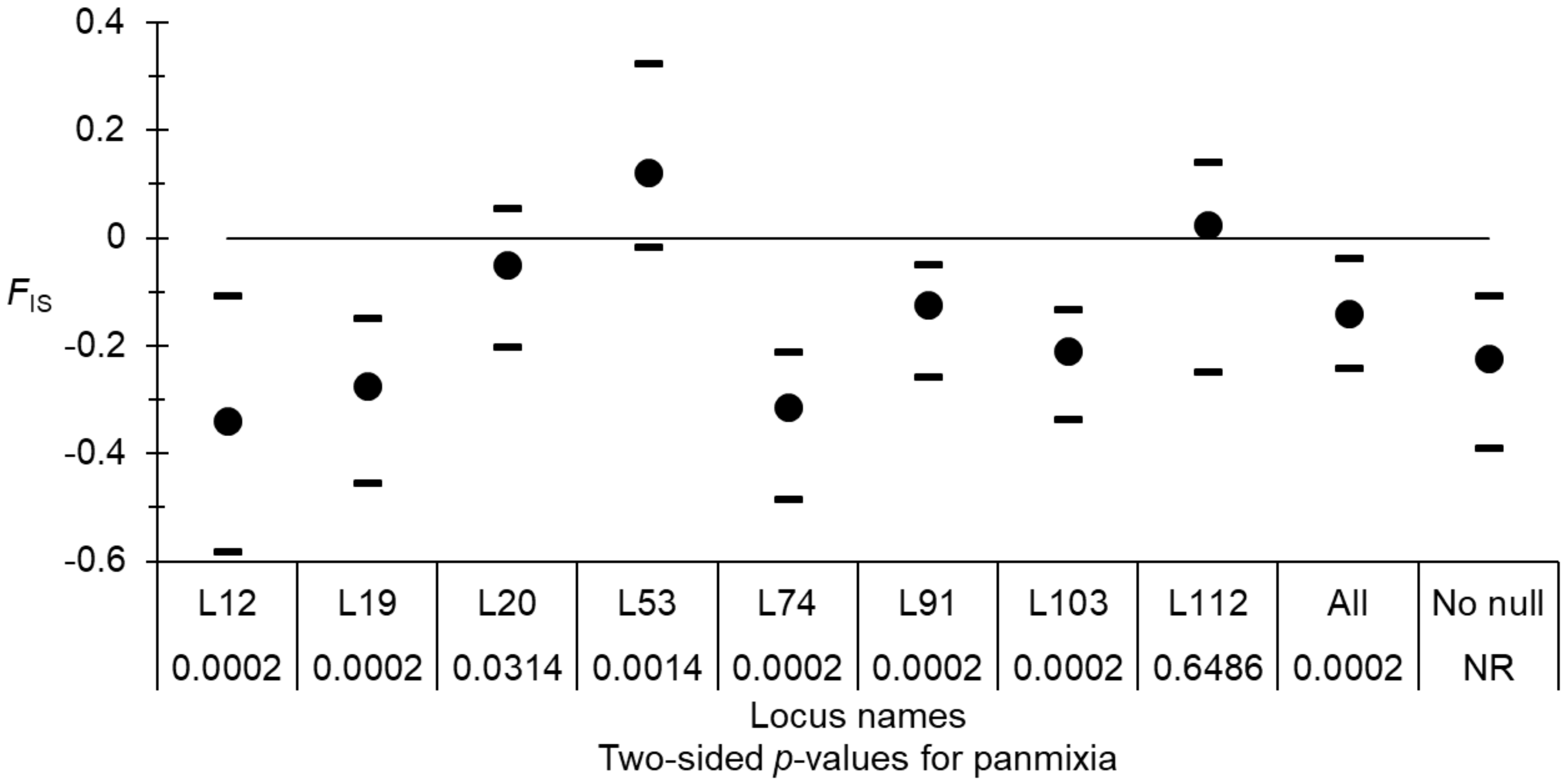
Only two locus pairs (7%) appeared in significant LD. None remained significant after BY correction. Overall, as expected for small dioecious populations, there was a significant heterozygote excess (Figure 2). Nevertheless, it varied considerably across loci (Figure 2). According to De Meeûs (2018) and Manangwa et al. (2019) null alleles could account for such variation.

Effective population sizes

In the western counties of Arizona, the average effective population size was N_e =84 with a minimax=[59, 110]. Assuming there were no other counties harboring ticks in Arizona but Cochise and Santa-Cruz, the total effective population size in this area could be considered as the double of N_e , thus N_{e -T}=2N_e =169 with a minimax=[118, 220]. Eastern counties displayed slightly higher and more variable values: N_e =175 with a minimax=[60, 337].

Genetic differentiation between eastern and western morphotypes

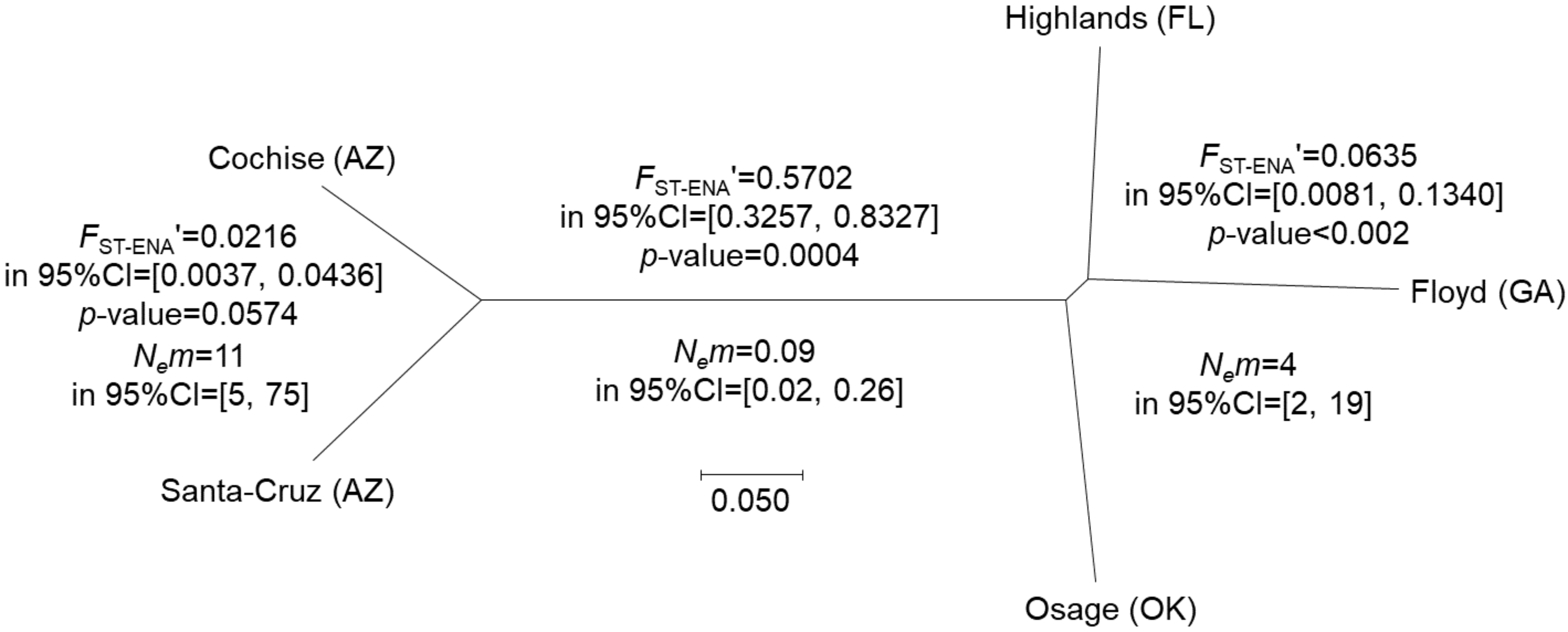
There were different degrees of genetic divergence between the counties and clades as illustrated by the NJTree (Figure 3). Subdivision was strong (F_ST-ENA′=0.5702 in 95%CI=[0.3257, 0.8327]) and very significant (p-value=0.0004) between the two morphotypes, translating into a very low number of immigrants (N_em=0.09, 95%CI=[0.0.0251, 0.2588]). Using the effective population sizes computed above, it was compatible with a split occurring about 234 generations ago with a 95%CI=[108, 504], and a minimax=[38, 1259]. If we consider a two year generation time, the estimates must be doubled.

Genetic differentiation within morphotypes

Figure 3 shows that there was a highly significant differentiation among eastern counties (p-value< 0.002) and a marginally not significant one (p-value< 0.0574) in Arizona, although the levels of subdivision and subsequent numbers of immigrants, overlap.

Isolation by distance

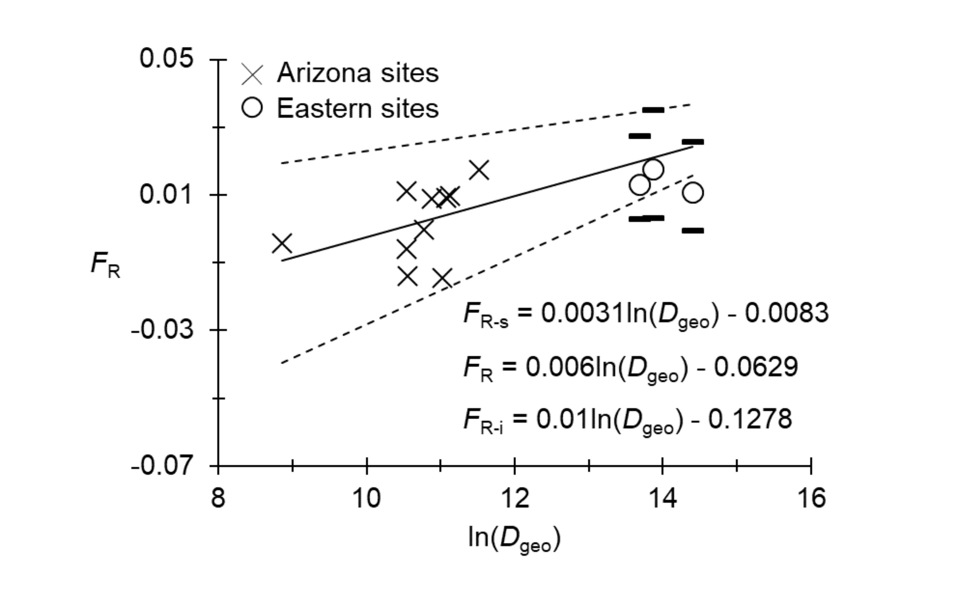
As illustrated in Figure 4, a significant isolation by distance appeared to occur among the Arizona sites. The test could not be performed for the East, because of the small number of sites. The small number of eastern points seemed; however, to align with the regression (Figure 4).

Dispersal distances

Using estimates of N_em between sites, the calculated average dispersal was δ=22 km per generation with 95%CI=[8, 52] (with the same minimax) in Arizona. Within eastern sites, dispersal was similar but with higher variance with δ=19 km per generation with 95%CI=[11, 163] and a minimax=[6, 473].

Effective population densities in Arizona

The isolation by distance slope (b) generated for Arizona (Figure 4) was used to infer a neighborhood of Nb=1/b=167 individuals with 95%CI=[100, 333] (Rousset 1997), which appeared to be very close to the total effective population size computed above (N_{e -T}=169). The number of immigrants exchanged between neighboring subpopulations was N_em=1/2πb=27 in 95%CI=[16, 53] per generation (Rousset 1997). The use of N_{e -T} resulted in small effective population density estimates of D_e =0.086 (95%CI=[0.060, 0.112]) individuals per km², with S_polygonAZ, and D_e =0.021 (95%CI=[0.015, 0.028]) with S_max. These computations resulted in an estimate of dispersal distances of δ=25 (95%CI=[19, 35]) with a minimax=[17, 42] km per generation (S_polygonAZ), or δ=50 (95%CI=[39, 71]) with a minimax=[34, 84] km per generation (S_max). These values are very close to those obtained with N_em between pairs of counties. Dispersal distances of 20-50 km per year (or every 2 years for a 2-year life cycle) appears, therefore, to be a robust estimate.

Bottleneck signatures

A significant bottleneck signature was found in each zone and each county with highly significant p-values for both the IAM and the TPM models; they were not significant for the SMM model. If we refer to Cornuet and Luikart (1996), with a H_S > 0.7, eight loci and around 30-40 individuals per county, we estimate that bottleneck detection required a α=N_{e -post}/N_{e -pre}=1000-fold population drop and parameter τ=g/(2N_{e -post})=1, where N_{e -post} and N_{e -pre} are the effective population sizes before and after the bottleneck, respectively, and g is the number of generations after the bottleneck. Assuming that the bottleneck coincided with the separation between the two clades (i.e., 234 generations,95% CI = [108, 504]), we computed an effective population size post bottleneck (N_{e PBN}) = 117 (95% CI = [54, 252]), which fits our N_e estimates (see above). This would indicate colonization events from a small number of ticks, 90 to 300 years ago, from a large ancestral population with N_{e -pre}\textgreater100,000 individuals.

Discussion

Here we found that the newly developed microsatellite markers of A. maculatum were informative at a U.S. scale. The markers showed none of the technical problems frequently occurring in ticks (De Meeûs et al. 2021). This study confirms that microsatellite markers can effectively replace occasionally noninformative mitochondrial and nuclear markers (Estrada-Peña et al. 2005; Lado et al. 2018) commonly used to delimit taxa, particularly for species that have evolved recently. Other genome-wide approaches (SNPs, for instance) are valid alternatives, but are still more costly than microsatellite analyses either because genomic sequencing requires important financial investment in equipment or expensive outsourcing. In addition, microsatellite loci can be amplified even from small amounts of genomic DNA, while SNP analyses require DNA samples of high quality and quantity.

The observed heterozygote excess was consistent with what is expected in small dioecious populations undergoing random mating (De Meeûs and Noûs 2023). In terms of population structure, we found an important subdivision between ticks from Arizona and those from the eastern United States. This subdivision appeared consistent with the existence of two species, which we named the Arizona and the Eastern clades, corresponding to the previously described morphotypes III and II, respectively. Lado et al. (2018) hypothesized ongoing or extremely recent speciation events driven by exposure to drastically different habitats (Cuervo et al. 2021). The observation that these two clades produce viable, albeit infertile, F1 offspring (Allerdice et al. 2020) further supports a recent radiation. The relatively recent origin of the two clades is confirmed by our estimate of the number of generations since divergence (234, 95%CI=(108, 504)). The length of the life cycle of A. maculatum s.s. is known to vary from one to two years depending on habitat and environmental conditions, with longevity increasing in the drier areas of Texas compared to relatively more humid localities in Oklahoma (Teel et al. 2010). Nothing is yet known about the life cycle length of the Arizona populations, but we can speculate that it would be similar to that observed in arid conditions. With a two-year life cycle, 234 generations would translate into 468 years. These are naturally approximations that must be considered cautiously. Nevertheless, they point to a recent common ancestor and divergence that may be driven by anthropogenic influences.

In each clade, we identified significant bottleneck signatures indicating that both clades likely originated from a relatively small number of colonizing ticks. Provided that the population of origin of the seeding ticks has not been submitted to important disturbances since the bottleneck event, we may predict that it should display a high effective population size of at least 100,000 individuals. We know that A. maculatum s.s. is found in Colombia (Ossa-López et al. 2022) and morphotype III in Mexico and that ticks of the group are often found on migratory birds flying northwards to the U.S. (Mukherjee et al. 2014). A better understanding of the population structure of A. maculatum s.l. in South and Central America could help to identify the origin of the U.S. populations.

The variance of dispersal distance estimates was much higher in the East than in Arizona. This may result from differences in the number of available sites (3 in the East and 5 in Arizona), the distances between sites (100 km max in AZ, 875 km min in the East), or may reflect ecological disparities. More eastern sites should therefore be sampled to clarify which hypothesis offers the most likely explanation. Nonetheless, in both clades, dispersal distances were high (between 20 and 60 km per generation). In Arizona, this suggests strong connectivity between the two counties, which would support a role of birds or wide-ranging mammals as regular hosts. Movement of cattle and dogs (Paddock and Goddard 2015; Nadolny and Gaff 2018) can cause similar displacements, but the frequent occurrence of such randomly directed events would probably have resulted in the progressive obliteration of the signature of isolation by distance. Because isolation by distance was significant, we consider anthropogenic movements of hosts to be less relevant in dispersing morphotype III ticks than wild animals.

The low densities of ticks found in Arizona (ie, a neighborhood size of approximately 167 individuals) suggest that these populations face difficult environmental conditions. Suitable habitats in Arizona are fragmented and confined generally to narrow riparian corridors within and among the Madrean Archipelago, an area surrounded by deserts. Indeed, consistently large and denser populations of morphotype III ticks have so far only been collected close to water (Lynn et al. 2024). It is premature to speculate on the future of such fragmented populations under climate change: either they (and their hosts) will progressively adapt to increasing aridity or face extinction. Estimates of population densities in the East will require sampling additional sites.

The Arizona and Eastern clades of A. maculatum ticks transmit R. parkeri (Paddock et al. 2004; Yaglom et al. 2019), an emerging pathogen that, following the important increase of its vectors' distribution, has now been detected in regions of the US far beyond its historically recognized range (Phillips et al. 2020, Molaei et al. 2021). This pathogen has been detected in A. triste, A. maculatum s.s. and morphotype III (Nava et al. 2008; Paddock et al. 2010; Delgado-de la Mora et al. 2017; Allerdice et al. 2017; Hecht et al. 2020; Paddock et al. 2020). Different genotypes of R. parkeri have been described, and some of them appear to be specifically associated with different tick morphotypes (Allerdice et al. 2021). The importance of determining the taxonomic status of A. maculatum s.l. populations in the U.S. is therefore not only of systematic interest but also public health relevance. Not only do the two morphotypes carry different genotypes of R. parkeri, but they are also characterized by different phenologies, as described recently (Lynn et al. 2024). This implies that disease risk assessments will also have to be tailored to the distinct life cycles of each morphotype.

Finally, because A. triste and A. tigrinum are very closely related to A. maculatum (Estrada-Peña et al. 2005; Lado et al. 2018), one would expect that they might share some microsatellite loci. It would certainly be interesting to test these markers on all clades identified in Lado et al. (2018) because species delimitations in this group of ticks could be improved by a reassessment of structure among South American populations.

Acknowledgements

We would like to thank Drs. Scott Harrison and Lance Durden, for their constructive comments about B.D.'s thesis, source of this publication. We would also like to acknowledge David Delgado-de la Mora, Jésus Delgado-de la Mora, and Jésus Licona-Enrîquez, for their contributions during field work. Dr Scot E. Dowd at MrDNA kindly helped us overcome bioinformatic issues. The editor's constructive critical review is also acknowledged.

References

1. Alkishe A., Peterson A.T. 2022. Climate change influences on the geographic distributional potential of the spotted fever vectors Amblyomma maculatum and Dermacentor andersoni. PeerJ, 10: e13279. https://doi.org/10.7717/peerj.13279
2. Allerdice M.E. 2021. Systematics and population structure of Amblyomma maculatum group ticks and Rickettsia parkeri, an emerging human pathogen in southern Arizona, USA [PhD Thesis]. Mississippi State, Mississippi State University. pp. 152. https://scholarsjunction.msstate.edu/td/5371
3. Allerdice M.E.J., Beati L., Yaglom H., Lash R.R., Delgado-de La Mora J., Licona-Enriquez J.D., Delgado-de La Mora D., Paddock C.D. 2017. Rickettsia parkeri (Rickettsiales: Rickettsiaceae) detected in ticks of the Amblyomma maculatum (Acari: Ixodidae) group collected from multiple locations in Southern Arizona. J. Med. Entomol., 54(6): 1743-1749. https://doi.org/10.3201/eid2504.181507
4. Allerdice M.E.J., Paddock C.D., Hecht J.A., Goddard J., Karpathy S.E. 2021. Phylogenetic differentiation of Rickettsia parkeri reveals broad dispersal and distinct clustering within North American strains. Microbiol. Spectr., 9(2): e0141721. https://doi.org/10.1128/Spectrum.01417-21
5. Allerdice M.E.J., Snellgrove A.N., Hecht J.A., Hartzer K., Jones E.S., Biggerstaff B.J., Ford S.L., Karpathy S.E., Delgado-de La Mora J., Delgado-de La Mora D., Licona-Enriquez J.D., Goddard J., Levin M.L., Paddock C.D. 2020. Reproductive incompatibility between Amblyomma maculatum (Acari: Ixodidae) group ticks from two disjunct geographical regions within the USA. Exp. Appl. Acarol., 82(4): 543-557. https://doi.org/10.1007/s10493-020-00557-4
6. Bajwa W.I., Tsynman L., Egizi A.M., Tokarz R., Maestas L.P., Fonseca D.M. 2022. The Gulf Coast tick, Amblyomma maculatum (Ixodida: Ixodidae), and spotted fever group Rickettsia in the highly urbanized northeastern United States. J. Med. Entomol., 59(4): 1434-1442. https://doi.org/10.1093/jme/tjac053
7. Beati L., Keirans J.E. 2001. Analysis of the systematic relationships among ticks of the genera Rhipicephalus and Boophilus (Acari: Ixodidae) based on mitochondrial 12S ribosomal DNA gene sequences and morphological characters. J. Parasitol., 87(1): 32-48. https://doi.org/10.1645/0022-3395(2001)087%5B0032:AOTSRA%5D2.0.CO;2
8. Beati L., Nava S., Burkman E.J., Barros-Battesti D.M., Labruna M.B., Guglielmone A.A., Cáceres A.G., Guzmán-Cornejo C.M., León R., Durden L.A., Faccini J.L. 2013. Amblyomma cajennense (Fabricius, 1787) (Acari: Ixodidae), the Cayenne tick: phylogeography and evidence for allopatric speciation. BMC Evol. Biol., 13(1): 267. https://doi.org/10.1186/1471-2148-13-267
9. Belkhir K., Borsa P., Chikhi L., Raufaste N., Bonhomme F. 2004. GENETIX 4.05, logiciel sous Windows ^TM pour la génétique des populations. Laboratoire Génome, Populations, Interactions, CNRS UMR 5171, Université de Montpellier II, Montpellier (France). https://kimura.univ-montp2.fr/genetix/
10. Benjamini Y., Yekutieli D. 2001. The control of the false discovery rate in multiple testing under dependency. Ann. Stat., 29(4). https://doi.org/10.1214/aos/1013699998
11. Cavalli-Sforza L.L., Edwards A.W.F. 1967. Phylogenetic analysis: models and estimation procedures. Evolution, 21(3): 550-570. https://doi.org/10.2307/2406616
12. Chapuis M.-P., Estoup A. 2007. Microsatellite null alleles and estimation of population differentiation. Mol. Biol. Evol., 24(3): 621-631. https://doi.org/10.1093/molbev/msl191
13. Cooley R.A., Kohls G.M. 1944. The Genus Amblyomma (Ixodidae) in the United States. J. Parasitol., 30(2): 77. https://doi.org/10.2307/3272571
14. Coombs J.A., Letcher B.H., Nislow K.H. 2008. CREATE: a software to create input files from diploid genotypic data for 52 genetic software programs. Mol. Ecol. Resour., 8(3): 578-580. https://doi.org/10.1111/j.1471-8286.2007.02036.x
15. Cornuet J.M., Luikart G. 1996. Description and power analysis of two tests for detecting recent population bottlenecks from allele frequency data. Genetics, 144: 2001-2014. https://doi.org/10.1093/genetics/144.4.2001
16. Cuervo P.F., Flores F.S., Venzal J.M., Nava S. 2021. Niche divergence among closely related taxa provides insight on evolutionary patterns of ticks. J. Biogeogr., 48(11): 2865-2876. https://doi.org/10.1111/jbi.14245
17. Delgado-de la Mora J., Sánchez-Montes S., Lincona-Énriquez J.D., Delgado-de la Mora D., Paddock C.D., Beati L., Colunga-Salas P., Guzmán-Cornejo C., Zambrano M.L., Karpathy S.E., López-Pérez A.M., Álvarez-Hernández G. 2019. Rickettsia parkeri and Candidatus Rickettsia andeanae in ticks of the Amblyomma maculatum group, Mexico. Emerg Infect Dis, 25: 836-838. https://doi.org/10.3201/eid2504.181507
18. De Meeûs, T. 2014. Statistical decision from k test series with particular focus on population genetics tools: a DIY notice. Infect. Genet. Evol., 22: 91-93. https://doi.org/10.1016/j.meegid.2014.01.005
19. De Meeûs, T. 2021. Initiation à la génétique des populations naturelles : applications aux parasites et à leurs vecteurs. 2ème édition revue et augmentée. IRD Editions, Marseille. https://doi.org/10.4000/books.irdeditions.40492
20. De Meeûs, T. 2018. Revisiting F_IS, F_ST, Wahlund effects, and null alleles. J. Hered., 109: 446-456. https://doi.org/10.1093/jhered/esx106
21. De Meeûs T., Beati L., Delaye C., Aeschlimann A., Renaud F. 2002. Sex-biased genetic structure in the vector of Lyme Disease, Ixodes ricinus. Evolution, 56(9): 1802-1807. https://doi.org/10.1111/j.0014-3820.2002.tb00194.x
22. De Meeûs T., Chan C.T., Ludwig J.M., Tsao J.I., Patel J., Bhagatwala J., Beati L. 2021. Deceptive combined effects of short allele dominance and stuttering: an example with Ixodes scapularis, the main vector of Lyme disease in the U.S.A. Peer Community J., 1. https://doi.org/10.24072/pcjournal.34
23. De Meeûs T., Guégan J.-F., Teriokhin A.T. 2009. MultiTest V.1.2, a program to binomially combine independent tests and performance comparison with other related methods on proportional data. BMC Bioinformatics, 10(1): 443. https://doi.org/10.1186/1471-2105-10-443
24. De Meeûs T., Humair P.-F., Grunau C., Delaye C., Renaud F. 2004. Non-Mendelian transmission of alleles at microsatellite loci: an example in Ixodes ricinus, the vector of Lyme disease. Int. J. Parasitol., 34(8): 943-950. https://doi.org/10.1016/j.ijpara.2004.04.006
25. De Meeûs T., Koffi B.B., Barré N., de Garine-Wichatitsky M., Chevillon C. 2010. Swift sympatric adaptation of a species of cattle tick to a new deer host in New-Caledonia. Infect. Genet. Evol., 10, 976-983. https://doi.org/10.1016/j.meegid.2010.06.005
26. De Meeûs T., McCoy K.D., Prugnolle F., Chevillon C., Durand P., Hurtrez-Boussès S., Renaud F. 2007. Population genetics and molecular epidemiology or how to "débusquer la bête″. Infect. Genet. Evol., 7(2): 308-332. https://doi.org/10.1016/j.meegid.2006.07.003
27. De Meeûs T., Noûs C. 2022. A simple procedure to detect, test for the presence of stuttering, and cure stuttered data with spreadsheet programs. Peer Community J., 2. https//doi.org/10.24072/pcjournal.165 https://doi.org/10.24072/pcjournal.165
28. De Meeûs T., Noûs C. 2023. A new and almost perfectly accurate approximation of the eigenvalue effective population size of a dioecious population: comparisons with other estimates and detailed proofs. Peer Community J., 3. https://doi.org/10.24072/pcjournal.280
29. Dempster A.P., Laird N.M., Rubin D.B. 1977. Maximum likelihood from incomplete data via the EM algorithm. J. R. Stat. Soc. Ser. B Methodol., 39(1): 1-38. https://doi.org/10.1111/j.2517-6161.1977.tb01600.x
30. Do C., Waples R.S., Peel D., Macbeth G.M., Tillett B.J., Ovenden J.R. 2014. NEESTIMATOR v2: re-implementation of software for the estimation of contemporary effective population size (N_e ) from genetic data. Mol. Ecol. Resour., 14(1): 209-214. https://doi.org/10.1111/1755-0998.12157
31. Estrada-Peña A., Venzal J.M., Mangold A.J., Cafrune M.M., Guglielmone A.A. 2005. The Amblyomma maculatum Koch, 1844 (Acari: Ixodidae: Amblyomminae) tick group: diagnostic characters, description of the larva of A. parvitarsum Neumann, 1901, 16S rDNA sequences, distribution and hosts. Syst. Parasitol., 60(2): 99-112. https://doi.org/10.1007/s11230-004-1382-9
32. Flenniken J.M., Tuten H.C., Rose Vineer H., Phillips V.C., Stone C.M., Allan B.F. 2022. Environmental drivers of Gulf Coast tick (Acari: Ixodidae) range expansion in the United States. J. Med. Entomol., 59(5): 1625-1635. https://doi.org/10.1093/jme/tjac091
33. Florin D.A., Brinkerhoff R.J., Gaff H., Jiang J., Robbins R.G., Eickmeyer W., Butler J., Nielsen D., Wright C., White A., Gimpel M.E., Richards A.L. 2014. Additional U.S. collections of the Gulf Coast tick, Amblyomma maculatum (Acari: Ixodidae), from the State of Delaware, the first reported field collections of adult specimens from the State of Maryland, and data regarding this tick from surveillance of migratory songbirds in Maryland. Syst. Appl. Acarol., 19(3): 257. https://doi.org/10.11158/saa.23.12.13
34. Goudet J. 1995. FSTAT (Version 1.2): A Computer Program to Calculate F-Statistics. J. Hered., 86(6): 485-486. https://doi.org/10.1093/oxfordjournals.jhered.a111627
35. Goudet J. 2003. FSTAT (version 2.9. 4), a program (for Windows 95 and above) to estimate and test population genetics parameters. Available at http://www.t-de-meeus.fr/Programs/Fstat294.zip (update from Goudet 1995). https://doi.org/10.1046/j.1365-294X.2002.01496.x
36. Goudet J., Raymond M., De Meeûs T., Rousset F. 1996. Testing differentiation in diploid populations. Genetics, 144(4): 1933-1940. https://doi.org/10.1093/genetics/144.4.1933
37. Guzmán-Cornejo C., Perez T.M., Nava S., Guglielmone A.A. 2006. Confirmation of the presence of Amblyomma triste Koch, 1844 (Acari: Ixodidae) in Mexico. Syst. Appl. Acarol., 11(1): 47. https://doi.org/10.11158/saa.11.1.5
38. Hasle G., Røed K.H., Leinaas H.P. 2008. Multiple paternity in Ixodes ricinus (Acari: Ixodidae), assessed by microsatellite markers. J. Parasitol., 94(2): 345-347. https://doi.org/10.1645/GE-1280.1
39. Hecht J.A., Allerdice M.E.J., Karpathy S.E., Yaglom H.D., Casal M., Lash R.R., Delgado-de La Mora J., Licona-Enriquez J.D., Delgado-de La Mora D., Groschupf K., Mertins J.W., Moors A., Swann D.E., Paddock C.D. 2020. Distribution and occurrence of Amblyomma maculatum sensu lato (Acari: Ixodidae) and Rickettsia parkeri (Rickettsiales: Rickettsiaceae), Arizona and New Mexico, 2017-2019. J. Med. Entomol., 57(6): 2030-2034. https://doi.org/10.1093/jme/tjaa130
40. Hedrick P.W. 2005. A standardized genetic differentiation measure. Evolution, 59(8): 1633-1638. https://doi.org/10.1111/j.0014-3820.2005.tb01814.x
41. Hijmans R.J., Williams E., Vennes C. 2019. Package ''geosphere'': spherical trigonometry. CRAN, pp. Spherical trigonometry for geographic applications. That is, compute distances and related measures for angular (Longitude/latitude) locations.
42. Keirans J.E., Durden L.A. 1998. Illustrated key to nymphs of the tick genus Amblyomma (Acari: Ixodidae) found in the United States. J. Med. Entomol., 35(4): 489-495. https://doi.org/10.1093/jmedent/35.4.489
43. Kempf F., De Meeûs T., Vaumourin E., Noel V., Taragel′ová V., Plantard O., Heylen D.J.A., Eraud C., Chevillon C., McCoy K.D. 2011. Host races in Ixodes ricinus, the European vector of Lyme borreliosis. Infect. Genet. Evol., 11(8): 2043-2048. https://doi.org/10.1016/j.meegid.2011.09.016
44. Kinsey A.A., Durden L.A., Oliver J.H. 2000. Tick infestation of birds in coastal Georgia and Alabama. J. Parasitol., 86(2): 251-254. https://doi.org/10.1645/0022-3395(2000)086%5B0251:TIOBIC%5D2.0.CO;2
45. Kohls G.M. 1956. Concerning the identity of Amblyomma maculatum, A. tigrinum, A. triste, and A. ovatum of Koch, 1844 (Acarina, Ixodidae). Proc. Entomol. Soc. Wash., 58: 143-147.
46. Kumar S., Stecher G., Tamura K. 2016. MEGA7: Molecular Evolutionary Genetics Analysis Version 7.0 for Bigger Datasets. Mol. Biol. Evol., 33(7): 1870-1874. https://doi.org/10.1093/molbev/msw054
47. Labruna M.B., Naranjo V., Mangold A.J., Thompson C., Estrada-Peña A., Guglielmone A.A., Jongejan F., De La Fuente J. 2009. Allopatric speciation in ticks: genetic and reproductive divergence between geographic strains of Rhipicephalus (Boophilus) microplus. BMC Evol. Biol., 9(1): 46. https://doi.org/10.1186/1471-2148-9-46
48. Lado P., Nava S., Mendoza-Uribe L., Caceres A.G., Delgado-de La Mora J., Licona-Enriquez J.D., Delgado-de La Mora D., Labruna M.B., Durden L.A., Allerdice M.E.J., Paddock C.D., Szabó M.P.J., Venzal J.M., Guglielmone A.A., Beati L. 2018. The Amblyomma maculatum Koch, 1844 (Acari: Ixodidae) group of ticks: phenotypic plasticity or incipient speciation? Parasit. Vectors, 11(1): 610. https://doi.org/10.1186/s13071-018-3186-9
49. Lynn G.E., Ludwig T.J., Allerdice M.E., Paddock C.D., Grisham B.A., Lenhart P.A., Teel P.D., Johnson T.L. The natural history of Amblyomma maculatum sensu lato, a vector of Rickettsia parkeri rickettsiosis, in southern Arizona. Sci. Rep., 14, 28175 (2024). https://doi.org/10.1038/s41598-024-78507-y
50. Manangwa O., De Meeûs T., Grébaut P., Ségard A., Byamungu M., Ravel S. 2019. Detecting Wahlund effects together with amplification problems: Cryptic species, null alleles and short allele dominance in Glossina pallidipes populations from Tanzania. Mol. Ecol. Resour., 19(3): 757-772. https://doi.org/10.1111/1755-0998.12989
51. McCoy K.D., Tirard C., Michalakis Y. 2003. Spatial genetic structure of the ectoparasite Ixodes uriae within breeding cliffs of its colonial seabird host. Heredity, 91(4): 422-429. https://doi.org/10.1038/sj.hdy.6800339
52. Meirmans P.G. 2006. Using the amova framework to estimate a standardized genetic differentiation measure. Evolution, 60(11): 2399-2402. https://www.jstor.org/stable/4134847 https://doi.org/10.1111/j.0014-3820.2006.tb01874.x
53. Mertins J.W., Moorhouse A.S., Alfred J.T., Hutcheson H.J. 2010. Amblyomma triste (Acari: Ixodidae): new North American collection records, including the first from the United States. J. Med. Entomol., 47(4): 536-542. https://doi.org/10.1093/jmedent/47.4.536
54. Molaei G., Little E.A.H., Khalil N., Ayres B.N., Nicholson W.L., Paddock C.D. 2021. Established population of the Gulf Coast tick, Amblyomma maculatum (Acari: Ixodidae), infected with Rickettsia parkeri (Rickettsiales: Rickettsiaceae), in Connecticut. J. Med. Entomol., 58(3): 1459-1462. https://doi.org/10.1093/jme/tjaa299
55. Mukherjee N., Beati L., Sellers M., Burton L., Adamson S., Robbins R.G., Moore F., Karim S. 2014. Importation of exotic ticks and tick-borne spotted fever group rickettsiae into the United States by migrating songbirds. Ticks Tick-Borne Dis., 5(2): 127-134. https://doi.org/10.1016/j.ttbdis.2013.09.009
56. Nadolny R.M., Gaff H.D. 2018. Natural history of Amblyomma maculatum in Virginia. Ticks Tick-Borne Dis., 9(2): 188-195. https://doi.org/10.1016/j.ttbdis.2017.09.003
57. Nava S., Elshenawy Y., Eremeeva M.E., Sunmer J.W., Mastropaulo M., Paddock C.D. 2008. Rickettsia parkeri in Argentina. Emerg Infect Dis, 14: 1894-1897. https://doi.org/10.3201/eid1412.080860
58. Nomura T. 2008. Estimation of effective number of breeders from molecular coancestry of single cohort sample: Estimation of effective number of breeders. Evol. Appl., 1(3): 462-474. https://doi.org/10.1111/j.1752-4571.2008.00015.x
59. Ogrzewalska M., Bajay M.M., Schwarcz K., Bajay S.K., Telles M.P.C., Pinheiro J.B., Zucchi M.I., Pinter A., Labruna M.B. 2014. Isolation and characterization of microsatellite loci from the tick Amblyomma aureolatum (Acari: Ixodidae). Genet. Mol. Res., 13(4): 9622-9627. https://doi.org/10.4238/2014.November.14.6
60. Ossa-López P.A., Robayo-Sánchez L.N., Uribe J.E., Ramírez-Hernández A., Ramírez-Chaves H.E., Cortés-Vecino J.A., Rivera-Páez F.A. 2022. Extension of the distribution of Amblyomma triste Koch, 1844: morphological and molecular confirmation of Morphotype I in Colombia. Ticks Tick-Borne Dis., 13(3): 101923. https://doi.org/10.1016/j.ttbdis.2022.101923
61. Paddock C.D., Sumner J.W., Comer J.A., Zaki S.R., Goldsmith C.S., Goddard J., McLellan S.L.F., Tamminga C.L., Ohl C.A. 2004. Rickettsia parkeri: a newly recognized cause of spotted fever rickettsiosis in the United States. Clin. Infect. Dis., 38(6): 805-811. https://doi.org/10.1086/381894
62. Paddock C.D., Fournier P.-E., Sumner J.W., Goddard J., Elshenawy Y., Metcalfe M.G., Loftis A.D., Varela-Stokes A. 2010. Isolation of Rickettsia parkeri and identification of a novel spotted fever group Rickettsia sp. from Gulf Coast Ticks (Amblyomma maculatum) in the United States. Appl. Environ. Microbiol., 76(9): 2689-2696. https://doi.org/10.1128/AEM.02737-09
63. Paddock C.D., Goddard J. 2015. The evolving medical and veterinary importance of the Gulf Coast tick (Acari: Ixodidae). J. Med. Entomol., 52(2): 230-252. https://doi.org/10.1093/jme/tju022
64. Paddock C.D., Hecht J.A., Green A.N., Waldrup K.A., Teel P.D., Karpathy S.E., Johnson T.L. 2020. Rickettsia parkeri (Rickettsiales: Rickettsiaceae) in the Sky Islands of West Texas. J. Med. Entomol., 57(5), 1582-1587. https://doi.org/10.1093/jme/tjaa059
65. Peel D., Waples R.S., Macbeth G.M., Do C., Ovenden J.R. 2013. Accounting for missing data in the estimation of contemporary genetic effective population size (N_e ). Mol. Ecol. Resour., 13(2): 243-253. https://doi.org/10.1111/1755-0998.12049
66. Phillips V.C., Zieman E.A., Kim C.-H., Stone C.M., Tuten H.C., Jiménez F.A. 2020. Documentation of the expansion of the Gulf Coast tick (Amblyomma maculatum) and Rickettsia parkeri: first report in Illinois. J. Parasitol., 106(1): 9-13. https://doi.org/10.1645/19-118
67. Piry, S., Luikart, G., Cornuet, J.M. (1999) BOTTLENECK: A computer program for detecting recent reductions in the effective population size using allele frequency data. Journal of Heredity, 90, 502-503. https://doi.org/10.1093/jhered/90.4.502
68. Ramírez-Garofalo J.R., Curley S.R., Field C.E., Hart C.E., Thangamani S. 2022. Established populations of Rickettsia parkeri- infected Amblyomma maculatum ticks in New York City, New York, USA. Vector-Borne Zoonotic Dis., 22(3): 184-187. https://doi.org/10.1089/vbz.2021.0085
69. R-Core-Team. 2022. R: a language and environment for statistical computing. 4.2.2 (2022-10-31 ucrt) ed. R Foundation for Statistical Computing, Vienna, Austria. https://www.R-project.org/
70. Rousset F. 1997. Genetic differentiation and estimation of gene flow from F -statistics under isolation by distance. Genetics, 145(4): 1219-1228. https://doi.org/10.1093/genetics/145.4.1219
71. Saitou N., Nei M. 1987. The neighbor-joining method: a new method for reconstructing phylogenetic trees. Mol. Biol. Evol., 4(4): 406-425. https://doi.org/10.1093/oxfordjournals.molbev.a040454
72. Scott J.D., McKeown J.T.A., Scott C.M. 2023. Migratory songbirds transport Amblyomma longirostre and Amblyomma maculatum ticks to Canada. J. Biomed. Res. Environ. Sci., 4(2): 150-156. https://doi.org/10.37871/jbres1659
73. Semtner P.J., Hair J.A. 1973. Distribution, seasonal abundance, and hosts of the Gulf Coast tick in Oklahoma. Ann. Entomol. Soc. Am., 66(6): 1264-1268. https://doi.org/10.1093/aesa/66.6.1264
74. Séré M., Thévenon S., Belem A.M.G., De Meeûs T. 2017. Comparison of different genetic distances to test isolation by distance between populations. Heredity, 119: 55-63. 10.1038/hdy.2017.26 https://doi.org/10.1038/hdy.2017.26
75. Sonenshine D.E. 2018. Range expansion of tick disease vectors in North America: implications for spread of tick-borne disease. Int. J. Environ. Res. Public. Health, 15(3): 478. https://doi.org/10.3390/ijerph15030478
76. Takezaki N., Nei M. 1996.Genetic distances and reconstruction of phylogenetic trees from microsatellite DNA. Genetics, 144(1): 389-399. https://doi.org/10.1093/genetics/144.1.389
77. Teel P.D., Hopkins S.W., Donahue W.A., Strey O.F. 1998. Population dynamics of immature Amblyomma maculatum (Acari: Ixodidae) and other ectoparasites on meadowlarks and northern bobwhite quail resident to the Coastal Prairie of Texas. J. Med. Entomol., 35(4): 483-488. https://doi.org/10.1093/jmedent/35.4.483
78. Teel P.D., Ketchum H.R., Mock D.E., Wright R.E., Strey O.F. 2010. The Gulf Coast tick: a review of the life history, ecology, distribution, and emergence as an arthropod of medical and veterinary importance. J. Med. Entomol., 47(5): 707-722. https://doi.org/10.1093/jmedent/47.5.707
79. Teriokhin A.T., De Meeûs T., Guegan J.F. 2007. On the power of some binomial modifications of the Bonferroni multiple test. Zhurnal Obshchei Biologii, 68, 332-340. PMID: 18038646
80. Trout R.T., Steelman C.D., Szalanski A.L., Loftin K. 2010. Establishment of Amblyomma maculatum (Gulf Coast Tick) in Arkansas, U.S.A. Fla. Entomol., 93(1): 120-122. https://doi.org/10.1653/024.093.0117
81. Velez R., De Meeûs T., Beati L., Younsi H., Zhioua E., Antunes S., Domingos A., Ataíde Sampaio D., Carpinteiro D., Moerbeck L., Estrada-Peña A., Santos-Silva M.M., Santos A.S. 2023. Development and testing of microsatellite loci for the study of population genetics of Ixodes ricinus Linnaeus, 1758 and Ixodes inopinatus Estrada-Peña, Nava and Petney, 2014 (Acari: Ixodidae) in the western Mediterranean region. Acarologia, 63(2): 356-372. https://doi.org/10.24349/bvem-4h49
82. Vitalis R., Couvet D. 2001a. Estimation of effective population size and migration rate from one- and two-locus identity measures. Genetics, 157(2): 911-925. https://doi.org/10.1093/genetics/157.2.911
83. Vitalis R., Couvet D. 2001b. Two-locus identity probabilities and identity disequilibrium in a partially selfing subdivided population. Genet. Res., 77(1): 67-81. https://doi.org/10.1017/S0016672300004833
84. Vitalis R., Couvet, D. 2001c. ESTIM 1.0: a computer program to infer population parameters from one- and two-locus gene identity probabilities. Molecular Ecology Notes, 1(4): 354-356. https://doi.org/10.1046/j.1471-8278.2001.00086.x https://doi.org/10.1046/j.1471-8278.2001.00086.x
85. Wang J. 2009. A new method for estimating effective population sizes from a single sample of multilocus genotypes. Mol. Ecol., 18(10): 2148-2164. https://doi.org/10.1111/j.1365-294X.2009.04175.x
86. Waples R.S. 2006. A bias correction for estimates of effective population size based on linkage disequilibrium at unlinked gene loci. Conserv. Genet., 7(2): 167-184. https://doi.org/10.1007/s10592-005-9100-y
87. Weir B.S., Cockerham C.C. 1984. Estimating F-statistics for the analysis of population structure. Evolution, 38(6): 1358. https://doi.org/10.2307/2408641
88. Wright S. 1965. The interpretation of population structure by F-statistics with special regard to systems of mating. Evolution, 19(3): 395. https://doi.org/10.2307/2406450
89. Yaglom H.D., Casal M., Carson S., O'Grady C.L., Dominguez V., Singleton Jr. J., Chung I., Lodge H., Paddock C.D. 2019. Expanding recognition of Rickettsia parkeri rickettsiosis in southern Arizona, 2016-2017. Vector-Borne Zoonotic Dis., 20(2): 82-87. https://doi.org/10.1089/vbz.2019.2491

instructions